Search This Blog


Trick or Trait

tl;dr

Scala’s traits are tricky. There are many pitfalls. especially, if you’re dealing with composed/stacked traits. I recently had an interesting conversation on whether it is best to extend a trait in another trait, or enforce a mixin with self typing (which apparently, can be done in several ways). This led me to some new findings (for me at least), and insights, on how and when to use the different approaches.

What’s wrong with the good old abstract class?

Scala has abstract classes, but they are limited. You cannot inherit more than one class or abstract class. Scala’s way to achieve “multiple inheritance” is via “trait mixins”. It also allows you to extend a trait with another trait, but according to the specs:

… A template \(sc \text{ with } mt_1 \text{ with } \ldots \text{ with } mt_n \{ stats \}\) consists of a constructor invocation \(sc\) which defines the template’s superclass, trait references \(mt_1,\ldots,mt_n (n≥0)\), which define the template’s traits, and a statement sequence stats which contains initialization code and additional member definitions for the template.

Each trait reference \(mt_i\) must denote a trait. By contrast, the superclass constructor \(sc\) normally refers to a class which is not a trait. It is possible to write a list of parents that starts with a trait reference, e.g. \(mt_1 \text{ with } \ldots \text{ with } mt_n\). In that case the list of parents is implicitly extended to include the supertype of \(mt_1\) as first parent type. The new supertype must have at least one constructor that does not take parameters. In the following, we will always assume that this implicit extension has been performed, so that the first parent class of a template is a regular superclass constructor, not a trait reference.

This is not something you would normally do. And there’s a good reason for it.

When should you use extends on a trait?

Scala’s traits are “stackable”, and can be used for “stackable modifications”. This feature is well blogged on, and not the main purpose of this current post, so go ahead and take a look at the basic example from Programming in Scala book.

The reason it works so well, is because each trait stacked extend IntQueue, and thus enforcing it’s own place in class linearization to the left of the implementing class, so super calls are always called in proper order. If we would not have extended, but merely enforce a mixin with self type, we wouldn’t be able to call super, thus not be able to stack operations.

import scala.collection.mutable.ArrayBuffer

abstract class IntQueue {
  def get(): Int
  def put(x: Int)
}

trait Doubling extends IntQueue {
  abstract override def put(x: Int) = { super.put(2 * x) }
}

trait Incrementing extends IntQueue {
  abstract override def put(x: Int) = { super.put(x + 1) }
}

// replacing definition with commented out
// self typing code won't compile:
//
// trait Filtering { this: IntQueue =>
trait Filtering extends IntQueue {
  abstract override def put(x: Int) = {
    if (x >= 0) super.put(x)
  }
}

class BasicIntQueue extends IntQueue {
  private val buf = new ArrayBuffer[Int]
  def get() = buf.remove(0)
  def put(x: Int) = { buf += x }
}

Usage:

scala> val q = new BasicIntQueue with Doubling with Filtering with Incrementing
q: BasicIntQueue with Doubling with Filtering with Incrementing = $anon$1@5e3dd1f3

scala> q.put(-3);q.put(0);q.put(-1);q.put(1)

scala> q.get()
res1: Int = 2

scala> q.get()
res2: Int = 0

scala> q.get()
res3: Int = 4

scala> q.get()
java.lang.IndexOutOfBoundsException: 0
  at scala.collection.mutable.ResizableArray.apply(ResizableArray.scala:46)
  at scala.collection.mutable.ResizableArray.apply$(ResizableArray.scala:45)
  at scala.collection.mutable.ArrayBuffer.apply(ArrayBuffer.scala:49)
  at scala.collection.mutable.ArrayBuffer.remove(ArrayBuffer.scala:173)
  at BasicIntQueue.get(IntQueue.scala:30)
  ... 36 elided

class linearization?

The specs define linearization according to the following formula:

$$ \mathcal{L}\big(\mathcal{C}\big)=\mathcal{C},\mathcal{L}\big(\mathcal{C_n}\big)\vec{+}\ldots\vec{+}\mathcal{L}\big(\mathcal{C_1}\big) $$

Where \(\vec{+}\) means you add new traits to the right, but only keep the right most appearance of the trait.

$$ \begin{alignat*}{3} a,A\vec{+}B&= a,\big(A\vec{+}B\big) && \textbf{ if }a\notin B \\\\ &= A\vec{+}B && \textbf{ if }a\in B \end{alignat*} $$

This means a class \(\mathcal{C}\), or in our case q, is linearized as:

val q = new BasicIntQueue with Doubling with Filtering with Incrementing

q = \(\mathcal{C}\)
BasicIntQueue = \(\mathcal{L}\big(\mathcal{C}_1\big)=\{BasicIntQueue,IntQueue,AnyRef,Any\}\)
Doubling = \(\mathcal{L}\big(\mathcal{C}_2\big)=\{Doubling,IntQueue,AnyRef,Any\}\)
Filtering = \(\mathcal{L}\big(\mathcal{C}_3\big)=\{Filtering,IntQueue,AnyRef,Any\}\)
Incrementing = \(\mathcal{L}\big(\mathcal{C}_4\big)=\{Incrementing,IntQueue,AnyRef,Any\}\)

$$ \begin{aligned} & q,\mathcal{L}\big(\mathcal{C}_4\big) \vec{+} \mathcal{L}\big(\mathcal{C}_3\big) \vec{+} \mathcal{L}\big(\mathcal{C}_2\big) \vec{+} \mathcal{L}\big(\mathcal{C}_1\big) \\ & q,\mathcal{L}\big(\mathcal{C}_4\big) \vec{+} \big(\mathcal{L}\big(\mathcal{C}_3\big) \vec{+} \big(\mathcal{L}\big(\mathcal{C}_2\big) \vec{+} \mathcal{L}\big(\mathcal{C}_1\big)\big)\big) \\ & q,Incrementing,\mathcal{L}\big(\mathcal{C}_3\big) \vec{+} \big(\mathcal{L}\big(\mathcal{C}_2\big) \vec{+} \mathcal{L}\big(\mathcal{C}_1\big)\big) \\ & q,Incrementing,Filtering,\mathcal{L}\big(\mathcal{C}_2\big) \vec{+} \mathcal{L}\big(\mathcal{C}_1\big) \\ & q,Incrementing,Filtering,Doubling,\mathcal{L}\big(\mathcal{C}_1\big) \\ & q,Incrementing,Filtering,Doubling,BasicIntQueue,IntQueue,AnyRef,Any \end{aligned} $$

Why should you care?

Well, to understand the subtle differences between extending or enforcing a mixin, you need to know about how class linearization is performed. Now, notice how when we defined the traits with extends, the linearization of that trait transitively contained the extended other trait. e.g: Doubling class linearization, contained IntQueue. This means, that as a user, no matter how I mix Doubling in my bottom type, in the linearization, IntQueue will always going to be found right to Doubling, and will always be the super. More importantly, IntQueue is going to be initialized prior to Doubling since initialization order takes effect from the right most element in the linearization, and advancing to the left. This is of-course not a problem with IntQueue case, and exactly what we want and expect, but sometimes, you would want to let the end user be in charge of initialization order.

The weird case of the val in the trait

As you probably know, traits are not interfaces. A trait can hold non abstract members, whether defs, vals, etc’… normally, you shouldn’t care about the linearization of your class. But if your traits interact with each other, and contain (possibly uninitialized) vals, you might (depends on how you defined your class hierarchy and inter-trait interaction) encounter some puzzling NullPointerExceptions. In these cases, since scalac prohibits any form of circular inheritance, a user can re-arrange mixins order of the bottom type, and carry on. Given of-course the user has full control of the class linearization. When you enforce a mixin using self typing, your trait, and the trait you enforce mixin with, can appear in any order once linearized. The user is in full control. And you can (though not necessarily should) use anything from the enforced mixin, as if it was “extended regularly”. As long as you also type alias this.

this aliasing?

this aliasing isn’t something new or unknown. There are many good reasons to do so1, but for now, just know there are several ways to do it, with very subtle differences between them.

trait A { self => ... }
trait A { self: B => ... }
trait A { this: B => ... }
trait A { _: B => ... }

In the first option, you give an alias to this, usually, so you would be able to refer to it from an inner class (which is quite handy if you utilize path dependent types). The second is interesting, it will force implementing classes to also mix in B trait. Options 3 & 4 are equivalent as much as I know (please correct me if I’m wrong).

conclusion

Adhering to the principle of least power, you should choose the most restrictive approach you can get by with. If all you need is to know your trait is always mixed with another trait2, use only a type (option 4). Also if you need to use another trait capabilities, but only from within a method, or in any way not during initialization, use self typing (options 2, 3, 4). If you also have inner classes and refers to this in the code, alias it as something else (convention is “self”) to ease readability. If you depend on another trait during initialization, then extend it to ensure correct ordering in class linearization. But do it only if you really must.


  1. maybe more on that in a future post.↩︎

  2. you may think what would be a good usecase. Well, I’m wondering about it myself. Maybe if you have a sealed trait, and you want the implementing classes to have some functionality, but you don’t want any other class to have that functionality and still want to put it in a different file. This way you enforce a trait from another file can only be mixed in with your sealed trait, and offer functionality without overloading too much logic in a single file. got any better idea? I’d love to hear :)↩︎
FP-ish patterns

Background

My twitter feed is becoming more and more (pure) FP oriented. Many of the people I follow from the Scala community are advocating for Haskell over Scala lately. To be honest, I was always intrigued about pure FP, but never got to use it in the “real world”1. I always worked in teams that had OOP mindset, and codebase. With Scala I was able to shift the balance a little bit towards FP. I advocated for referential transparency, strongly typed over stringly typed code, higher order functions, higher kinded types, typeclasses, etc’… I aimed to be more FP in an OO world. But I never managed to get my peers into learning together, and using, “pure FP” with libraries like cats or scalaz. So I wonder, does pure FP really is the answer - the silver bullet - I’m looking for, or should we tilt the balance less towards purity in Scala?

Harsh criticism against impure Scala

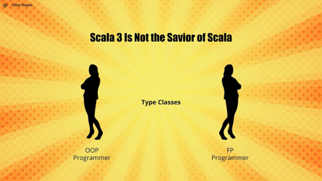
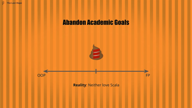
In the latest scalapeno conference, I attended John De Goes’ keynote “The Last Hope for Scala’s Infinity War”. In the talk, John claimed that: > “Some of the proposed features in Scala 3 are targeting someone who doesn’t exist”

He referred to features like Type Classes & Effect System. features for no one

But the truth is, that john was wrong. There is at least one person that wants such features2. There is a middle-ground. And I want to believe I’m not alone, and some other people see the value Scala has to offer for FP lovers (wannabes?) working with traditional OO programmers, trying to make a difference. neither

Like John, I love Scala. but unlike John, I don’t think we need to sacrifice half the community

And I don’t want to see all the crossed out features removed from Scala: liabilities?

Scala is expressive

I was recently asked, why I love Scala. I answered that with Scala, It’s very easy for me to express exactly what I mean for the program to do, and that it’s easy to expose beautiful (and safe) functional interface, while encapsulating impure logic and gaining the benefit of both worlds. I was then asked to give an example, of short code that I find easy to express in Scala, and hard(er) to write in other languages. I choose something I’ve written a while ago, and I find as a nice example for such FP-ish pattern.

def mapr[A,B](as:         Vector[A])
             (f:    A  => Future[B])
             (g: (B,B) => Future[B]): Future[B]

So… what’s so special about mapr? A quick scala thinker will implement it with something like3:

Future.traverse(as)(f)
      .flatMap(_ reduce g) // if g were (B,B) => B

And it can be fine, considering the usecase. It wasn’t fine in our case.

The “real world” case

Consider A to be file names to fetch from a S3 bucket. But not just any file, it’s a CSV with time series events. B is a time based aggregated states series of the events. f can be “fetch & aggregate” a single file. But since many “sources” (S3 files) can add data, we should think about merging (reducing) multiple sources into one uber states series4. Thus we need g to “merge” two time based aggregated states into a single time based state series. Now, file sizes range from a few MBs, up to ~10GB. And this is important, because in the simple solution, we cannot start reduce-ing the small files, until we are done fetching and transforming the bigger 10GB files. Also, if the first A in the Vector is also mapped to the heaviest B, the reduce will be expansive since we always merging ~10GB B.

Lawful properties

In this case, there are interesting things to note about g5:

  • g is assocciative, it doesn’t matter how we group and merge two time based series states.
  • g is commutative, order is irrelevant. switch LHS with RHS, and get exactly the same result.

So now, our random pure-FP dude might say: great! your category B sounds very similar to a semilattice. Let’s also prove that g abides the idempotency law, and that g(b,b) == b for any \(b\), and maybe we’ll find a useful abstraction using semilattice properties.

Well, that FP-programmer is actually right. and all that high gibberish talk actually has solid foundations. And in fact, that function g over B I just described does define a semilattice. Bs has partial ordering6, g acts as the “join” operation, and we even have an identity element (the empty time series), so it is even a “Bounded Semilattice”.

But this is totally irrelevant and out of the question’s scope. Remember, we are working in an OO organization. If we start defining abstractions over semilattices (or maybe there are ones in cats or scalaz libraries? I really don’t know), The code will become one giant pile of gibberish in the eyes of my coworkers. And we don’t even need it. What is needed, with the realization that g is associative & commutative, is a very natural optimization that pops to mind: why wait for all A => B transformations? whenever 2 Bs are ready, any 2 Bs, we can immediately apply g and start the merge process.

So, without over abstracting, I came up with the following piece of code (brace yourselves):

def unorderedMapReduce[A, B](as: Vector[A])
                            (f: A => Future[B], g: (B,B) => Future[B])
                            (implicit executor: ExecutionContext): Future[B] = {

  val promises = Array.fill(2 * in.size - 1)(Promise.apply[B])
  var i = 0 // used for iteration optimization
            // (not needing to search for uncompleted
            // promise from start every time)

  def completeNext(tb: Try[B]): Unit = tb match {
    case Failure(e) => promises.last.tryFailure(e) // fail fast
    case Success(b) =>
      // We're not synchronizing i, since we can guarantee we'll always
      // get an i that is less than or equal to latest i written by any
      // other thread. But we cannot use i += 1 inside the loop,
      // since it may result with skipping a cell in 2 threads doing
      // the increment in parallel, so each thread get's an initial copy
      // of i as j, and only increment it's own copy. eventually,
      // we replace i with a valid value j (less than or equal to
      // first not used promise)
      var j = i
      var p = promises(j)
      while ((p eq null) || !p.trySuccess(b)) {
        j += 1
        p = promises(j)
      }
      i = j
  }

  as.foreach { a =>
    f(a).onComplete(completeNext)
  }

  promises
    .init
    .zipWithIndex
    .sliding(2,2)
    .toSeq
    .foreach { twoElems =>
      val (p1, i1) = twoElems.head
      val (p2, i2) = twoElems.last

      // andThen side effect is meant to release potentially heavy
      // elements that otherwise may stay for potentially long time
      val f1 = p1.future.andThen { case _ => promises(i1) = null }
      val f2 = p2.future.andThen { case _ => promises(i2) = null }
      failFastZip(f1,f2)
        .flatMap(g.tupled)
        .onComplete(completeNext)
    }
  promises.last.future
}

// regular Future.zip flatMaps first future, so it won't
// fail fast when 2nd RHS future completes first as failure.
def failFastZip[A,B](l: Future[A], r: Future[B])
                    (implicit executor: ExecutionContext): Future[(A,B)] = {
  val p = Promise[(A,B)]()
  l.onComplete(_.failed.foreach(p.tryFailure))
  r.onComplete(_.failed.foreach(p.tryFailure))
  for {
    a <- l
    b <- r
  } p.success(a -> b)
  p.future
}

I can imagine the horror on the face of our random FP-dude, an Array (mutable), vars, nulls, side effects,… OMG. John would not approve such abomination. But before you panic, bare with me and let’s break it down.

The what & how

The goal is to have a “bucket” of ready B elements, and whenever we have 2 or more Bs in the “bucket”, we take a pair out of the bucket, compute g on it, and when g returns with a new B, we put it right back in the “bucket”, and we continue to do so, until only a single finite B element is left in the bucket. this is our return value.

The way it is done, is simple. we have \(n\) A elements in the original sequence, each will be mapped to a single B, and since every 2 Bs are used to generate a new B, we need room for another \(n-1\) Bs in the bucket. Overall, \(2n-1\) elements, and our “bucket” can be just a simple Array. We also want to parallelize the computation as much as we can, so some construct to handle the asynchronous nature of the computation is needed. I used a Promise[B] to store the result. So our “bucket” is simply an Array[Promise[B]] of size \(2n-1\).

Have a look at the following figure: pic This illustrates the order of computation, when the order is:

  1. as(2)
  2. as(1)
  3. g(as(2),as(1))
  4. as(3)
  5. as(0)
  6. g(g(as(2),as(1)),as(3))
  7. g(as(0),g(g(as(2),as(1)),as(3)))

In the simple FP approach (traverse + reduce), same execution will result with the following computation order:

  1. as(2)
  2. as(1)
  3. as(3)
  4. as(0)
  5. g(as(0,as(1))
  6. g(g(as(0,as(1)),as(2))
  7. g(g(g(as(0,as(1)),as(2)),as(3))

Which means we don’t take advantage of the early completed computations.

More benefits

Using early completed computations isn’t the only reason I argue the suggested code is superior. It’s not just we start computations eagerly, implicitly it also means that heavy elements are left to be dealt in in the end, and we don’t need to reduce 10GB files at every step of the way7. We also get “fail fast” semantics; for example, if g fails for whatever reason on as(2) input, in the code I suggest, you fail fast since it is mapped directly as a failed Future result. Also, whenever a future completes, we have a side effect to clean up values that are not needed anymore, so we don’t leak.

Bottom line

What I try to emphasize using the example I showed, is that there are good reasons to write impure functional code. In cases like this, you enjoy both worlds. The interface is functional, it is referential transparent (as much as Future is considered referential transparent). Perhaps the above is achievable using pure functional style (I would love to know how. really!), but my gut is telling me it won’t be so simple. And as someone who works mostly in hybrid FP-OO teams, I can’t go full FP. Not at first anyway… Using Scala enables me to introduce a smoother transition into FP without getting my peers too angry or confused. It enables me to break the rules if I really need to. I wouldn’t sacrifice the impure parts of the language. I truly think they are too valuable.


  1. Other than maybe a tiny PR to coursier which uses scalaz.↩︎

  2. You are reading that person’s blog. Obviously :)↩︎

  3. Actually, I’d bet he would use Traversable and Task over std lib’s Future.traverse↩︎

  4. There are multiple ways to approach that problem, and actually, we ended up with another solution, that utilized akka-streams, merging multiple sources with a custom stage & scaning to output a stream of aggregated state in time order.↩︎

  5. Whenever I encounter such realization, I automatically translate it to property checks tests. So to test that g is lawful, all I needed is a very simple scalacheck test to test associativity & commutativity.↩︎

  6. think about b1 != b2, which means that either g(b1,b2) > b1 and also g(b1,b2) > b2, or that b1 and b2 already has order relation between them. It may be more obvious in some situations (and it was obvious in our case).↩︎

  7. Kind of reminds me of the matrix chain multiplication problem.↩︎

The worst interview question

tl;dr

We, the software development industry people, seek new job opportunities every now and then. Those of us who are in the game long enough, have seen all kinds of interviews. Maybe even conducted interviews for others. As someone who has been on both sides of the fence, I’d like to share some insights, mostly aimed for those conducting the interview, and I’ll do it by sharing a real example.

Assume nothing

Every interview conductor has been interviewed by someone else at some point. This is how we get in. It seems like some people tend to forget how it looks from the other end of the table. When asking technical or theoretical questions, one should be very clear, and verify the person standing in front of him understood the question. More often than not, we assume people understand what we meant for them to understand, only to find out later it wasn’t the case. We also tend to assume people think similarly to us about the problems we present to them. Obviously, those assumptions are wrong.

The trick is to not use any tricks

When we ask a question, it should be clear to us what information can we infer on the candidate standing before us from the way he answers. Some questions has no value at all. Usually, “trick questions”, for example, has no value. Either the candidate knows the question, and the trick to solve it, or they don’t. Asking such question yields nothing meaningful if the candidate knows the answer by heart. And have little value if they don’t (you do get to see how they think, and how they approach the problem). Thing is, it hurts the candidate confidence if you present a question they fail to answer, and it will affect them for the rest of the interview. Some trick answers, are not even the (most) correct answers to the question. A (very) good candidate might know better, and a fixed minded interviewer, who has his mind set on the trick answer, might not understand it.

The worst interview question

I was once asked to solve such trick question. I also knew the trick and that it wasn’t the best approach. The question was (essentially1): > given a shuffled sequence of \(n - 1\) numbers, all distinct and part of an arithmetic sequence range of \(n\) numbers, find the missing number in the sequence.

There are many ways to answer that question. I will present 4 solutions in rising complexity order, but eventually, you will see that the simple solutions I discuss here have gentle flaws, and best answer, is actually the most complicated one. Disclaimer: after writing this post, it occured to me that there is an elgant and correct solution, simply XOR all the numbers and the full range itself. Since all numbers cancel each other, we are left with the one number in the range that is not present in the sequence. But neither I nor the interviewer have thought of that at the moment. Moreover, I feel it’s also important to note (though not the main goal of the post) that abstracting the question too much, like what was done here, only increases the gap between the understanding of the interviewer (and what he meant), and the understanding of the candidate2. Anyway, we are aiming for linear (time) complexity answer3.

1st Answer (the trick)

We are talking about an arithmetic sequence, so let’s use the formula: we can scan the sequence, and find \(min\), \(max\), & \(sum\) of given numbers, and compute the difference: $$result=\frac{n(min + max)}{2}-sum$$ Simple. Elegant. And flawed to the core! So what’s wrong with it? Well… The implicit assumption here, is that adding 2 numbers is done at constant time. Isn’t it? NO! it’s only constant if you use primitives such as 32 bit int, or 64 bit long, etc’… But we have no restrictions on the length of the given sequence. If we use primitives, we risk arithmetic overflow, and get a wrong answer. So we need to use something like BigInteger, which has addition operation in linear complexity with the numbers of digits (bits) of the number. I.e: logarithmic in terms of \(n\). So either it’s wrong, or we ended up with implicitly \(n\log(n)\) complexity.

2nd Answer

OK, let’s try again. we have an arithmetic sequence, so it means we have a bijective function4 \(f\) into \(\mathbb{N}\)5. This means we also have the reversed function \(f^{-1}\). We can initialize a boolean array a with size of \(n\) and false values in all cells. On the next step, we iterate over the original sequence, and for every number \(k\) we encounter, we compute the index \(i=f\big(k\big)\), and set a[i]=true. Once we are done, the boolean array will be filled with true values in all cells, besides in the cell corresponding to the missing number. We can easily iterate over that array, and find that index j, and compute the result with \(f^{-1}\big(j\big)\). Is this better? well… not so much… we basically traded our \(O\big(n\log(n)\big)\) time complexity and \(O\big(1\big)\) space complexity with linear time & space complexity. This feels like cheating. Trading time complexity with space complexity isn’t really improving. And we can easily think of scenarios where we don’t have the luxury of allocating so much memory.

3rd Answer

From now on I’m going to explain the solutions in terms of numbers in the range \(\big[1,n\big]\) instead of speaking about our bijective function \(f\) and it’s reversal \(f^{-1}\), for simplicity. Trying again, we can come up with a slightly more complex solution, but more “memory friendly” (pseudo code):

i,j ← 0
while(i < n - 1) {
  j ← a[i]
  while(j > i) {
    swap(a[i],a[j])
    j ← a[i]
    if(j == n) {
      return i
    }
  }
  i++
}
return n - 1

So what’s going on here? we scan the sequence a, and as long as a[i]==i we do nothing. When it’s not equal, it means it is larger6. In this case, we look at the cycle a[i] → a[a[i]] → … → i, and swap elements as we go until we finished the cycle, and all the elements we’ve seen, are now properly placed in their corresponding indices. There is one special “cycle” though. The “cycle” (list actually) containing \(n\) itself. This list will start with the missing element’s index, and will end when we reach the cell containing \(n\). Why? I’ll leave it as an exercise for you to figure out. you can check out the hint if you want7. So, is this better? well yes. but still not perfect. we still used an assumption implicitly, without realizing the question does not allow it. I’m talking about RAM. The ability to hop between indices back and fourth in \(O\big(1\big)\) time is not explicitly given, and we cannot assume it. In case we do have RAM access, we use \(O\big(n\big)\) time & \(O\big(1\big)\) space. So we’re half way there. But since in our world, we may talk about a linked model only (think about distributed graphs, scattered files on some cloud, etc’…), we can try to do better.

4th Answer

In this last answer, I’m gonna count on the reader having some basic CS 101 knowledge (don’t worry too much if you don’t, I’ll link to resources where necessary), and will only describe the idea in higher level, since it’s gonna be too terse to delve into all the lower level details. Take a moment to refresh your memory on quicksort algorithm. We’ll tear it apart, and use the building blocks to solve our problem. Wikipedia’s high level description of the algorithm is as follows:

  1. Pick an element, called a pivot, from the array.
  2. Partitioning: reorder the array so that all elements with values less than the pivot come before the pivot, while all elements with values greater than the pivot come after it (equal values can go either way). After this partitioning, the pivot is in its final position. This is called the partition operation.
  3. Recursively apply the above steps to the sub-array of elements with smaller values and separately to the sub-array of elements with greater values.

Wikipedia is speaking in terms of “array”, but quicksort also works perfectly well on linked lists. What we will do, is similar:

  1. Pick a GOOD pivot
  2. Use partition
  3. After partition, check if index(pivot) == pivot or index(pivot) == pivot - 1 8
  1. If equal recurse only on > pivot part of the sequence
  2. If pivot is larger (by 1) than it’s index, recurse only on < pivot part of the sequence
  1. When sequence is small enough (e.g. < 5), sort it, and check sorted sub-sequence together with next index’s element (if exist, could be a pivot from previous iteration). the gap will be there.

What are we aiming at here? well, before we go into complexity analysis, we need to explain why it works. It’s not a formal proof, but good enough. We know we have all the numbers except one in the range \(\big[1,n\big]\). And we know the indices are \(\big[1, \dots, n-1\big]\). So if we would’ve sorted the sequence, all the elements before the gap would’ve been found at the correct index (a[i] == i), and all the elements larger than the missing element would’ve been at an offset of one from their index (a[i - 1] == i). So if we place the pivot at exactly the correct index, we can tell by looking at the offset if we are higher or lower than the missing element. So we do something very similar to quickselect, only instead of knowing up front the index \(k\) we want, we iterate according to the index offset. When we finish, the gap might be at a neighboring cell (if missing element index was chosen as pivot at a previous round of the iteration), and we check \(O\big(1\big)\) sorted elements containing the gap for the missing element. I claim that if we choose a good pivot, this process will take linear time. But before I explain why, I’ll give you a minute to see that good pivots can be chosen in linear time. The tl;dr of it, is that we can choose a pivot that will be in the range \(\big[0.3n,0.7n\big]\), so we avoid the worst case leading to \(O\big(n^2\big)\) running time. in the worst case, we are always left with 70% of our sequence to check. Each iteration is \(O\big(n'\big)\) where \(n'\) is the size of the subsequence we iterate on. This is because choosing a good pivot takes \(O\big(n'\big)\) and partition takes another \(O\big(n'\big)\). in total, we’ll get $$\sum_{i=0}^{log_{10/7}{n}}{2{\Big(\frac{7}{10}\Big)}^{i}}n=2n\sum_{i=0}^{log_{10/7}{n}}{{\Big(\frac{7}{10}\Big)}^{i}}\lt2n\sum_{i=0}^{\infty}{{\Big(\frac{7}{10}\Big)}^{i}}=2n\cdot{3\frac{1}{3}}=O\big(n\big)$$

There is so much I’m not explaining here, and many short cuts taken (especially in the math). Like, why (and how) does it work on linked lists, why it’s OK to compare numbers and assume it’s \(O\big(1\big)\), but not ok to assume this for addition (actually, it’s not. but in the first solution we summed up \(n\) elements, meaning \(n^2\) must be less than our primitive max value. when we compare primitives without summing, we can use the entire primitives range [think of unsigned 64 bit long…], which is still better than using \(\sqrt{primitive\ max\ value}\) ), etc’… But I want to cut to the point.

The point

This is a very bad question to ask in job interviews. But what I wish for you to take from this, is not the fact that some questions are more suited than others for job interviews (well, that too). It is the fact that in most cases there is a huge gap between the candidate and the interviewer. I’m not talking about intelligence here. I’m talking about the fact that any question can be misunderstood very easily, as any answer can be misunderstood very easily as well9. So neither the interviewer, nor the candidate should be taken lightly. We tend to disrespect who we don’t understand too easy. Try to overcome the urge, and try to put yourselves in the other side of the table. Of course this is aimed more for the interviewer, than the candidate. And keep in mind, you as the interviewer, want to hire the best and smartest person for the job. So don’t be hasty and give up one someone who might be that perfect candidate. Force yourself to understand. And remember, in our industry, it’s very possible you’ll find yourself in the candidate shoes in the future.


  1. they did not actually use the term “arithmetic sequence” since that would give hint to the trick they were after. Instead, they gave a vague definition of numbers spaced evenly between two arbitrarily large numbers \(m\) & \(M\)↩︎

  2. candidate might understand exactly what he’s being asked. In this example, and since the interviewer was obviously after the trick answer, he could’ve present the question as numbers in the range \(\big[1,n\big]\), instead vaguely defining an arithmetic sequence without naming it↩︎

  3. because sorting in \(O\big(n\log{n}\big)\) and scanning for the gap is trivial, and we can obviously do better↩︎

  4. meaning one‑to‑one correspondence↩︎

  5. \(\mathbb{N}\) stands for the naturals numbers↩︎

  6. Why? well… let’s leave it as an exercise for the reader ;)↩︎

  7. This is not easy or trivial (even with the hint), and the only reason I’m leaving it out and not explaining in full, is because it’s not this post’s goal, and it is getting lengthier than I thought already.↩︎

  8. That’s the only 2 possible options.↩︎

  9. And as you probably understand, this is exactly what happened to me on that occasion. I should’ve taken the understanding gap into consideration.↩︎